In the first article of this series, we studied Einstein, Podolski and Rosen’s paper, where we encountered for the first time the concept of quantum entangled stated and their “spooky action at a distance”.

As EPR realized, when particles interact (under certain conditions), a new type of non-classical correlations arise. In order to understand why entangled states concerned Einstein so much, you have to remember that he never accepted the Copenhagen Interpretation of Quantum Mechanics. Among many other things, this interpretation postulated that physical observable properties arise only when they are measured, meaning that the interaction of an apparatus (observer) and the systems causes the wave-function to collapse. A perfect example of this is the so-famous Schrödinger Cat Experiment (I won’t get into any detail as I’m sure you all know what I’m talking about).

Schrodinger's Cat

However, Einstein believed that in any complete physical theory, one should be able to predict the values of observable properties of quantum systems without the need to perform any measurement or to disturb the system. Said otherwise, physical observable properties should exist and have definite values independent of observation, they should be elements of reality. This is stated explicitly in EPR’s criterion of reality and sometimes recalled in Einstein’s quote:

“I, at any rate, am convinced that He (God) does not throw dice.”

-A. Einstein

In this article we will continue to study quantum entangled states and we will see what was the fundamental mistakes that Einstein, Podolski and Rosen made in the derivation of their “paradox”. Also, we will show why it is that we say that these correlations between quantum systems cannot be accounted for by any classical theory.

Bell’s Inequalities

Twenty nine years after EPR’s paper was published, John S. Bell, an Irish physicist working at CERN published a paper entitled “On the Einstein-Podolski-Rosen Paradox“. In his work, Bell proposed an experiment that could, once and for all, disprove EPR’s paradox. The main results of his paper are now known as Bell’s Inequalities.

In order to understand said results we have to first work in a classical framework. Consider the following thought experiment: two entangled particles are prepared and each is sent to a different observer (let’s call them Alice and Bob). When Alice receives her particle, she decides to perform a measurement on it. To do so, she has two available devices, and she can randomly choose between them to decide which one to use. The first device can measure a physical property M and the second one a physical property N. For simplicity’s sake, lets suppose that each measurement has only two possible outcomes: $\pm 1$ .

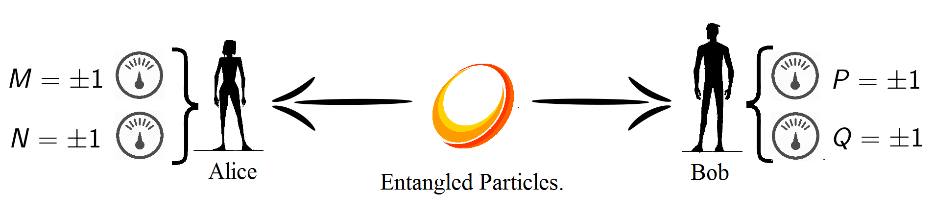
The same goes for Bob as he is capable of measuring one of these two properties: P or Q. Just like before, the possible outcomes for Bob’s measurements are $\pm 1$ . Let’s also say that Alice and Bob time their measurements so they perform them at the exact same time (said otherwise, none has any knowledge of either the measurement device selected nor the outcome obtained by the other one), thus being casually disconnected.

Let’s consider the following equation:

$MP+NP+NQ-MQ=(M+N)P + (N-M)Q$ . (1)

It’s easy to see that either $(M+N)=0$ or $(N-M)=0$ , and therefore $MP+NP+NQ-MQ=\pm 2$ . Next, we want to determine the probability $p(m,n,p,q)$ that the particles were created in a state such that $M=m$ , $N=n$ , $P=p$ and $Q=q$ . The mean value of this quantity is $E(MP+NP+NQ-MQ)$ , and can be calculated as

$\sum_{mnpq} p(m,n,p,q) (mp+np+nq-mq)\leq \sum_{mnpq} 2 \times p(m,n,p,q)$ (2.1)

$\leq 2$ . (2.2)

Which can also be written as

$\sum_{mnpq}p(m,n,p,q)mp+p(m,n,p,q)np+p(m,n,p,q)nq-p(m,n,p,q)mq$ (3.1)

$=E(MP)+E(NP)+E(NQ)-E(MQ)$ . (3.2)

From Eq. (2.2) and (3.2) we obtain

$E(MP)+E(NP)+E(NQ)-E(MQ) \leq 2$ . (4)

Equation (4) is one of Bell’s Inequalities, and it’s often called as the CHSH inequality (after John Clauser, Michael Horne, Abner Shimony, and Richard Holt). Experimentally, Alice and Bob can determine the values of $E(MN+NP+NQ-MQ)$ by repeating the experiment multiple times. Before proceeding, it’s important to remember that in order to obtain Eq. (4) we didn’t use Quantum Mechanics, Eq. (4) presents a constraint on the statistics of coincidences in the experiment.

Let’s go back to Quantum Mechanics, and suppose that the particles are prepared on the state

$|\psi\rangle=\frac{|\downarrow\uparrow\rangle-|\uparrow\downarrow\rangle}{\sqrt{2}}$ , (5)

(as we saw in my previous article, $|\psi\rangle$ is an entangled spin state), and suppose that Bob and Alice want to measure the following observables

$M=S^z_1, \qquad P=\frac{-S^z_2-S^x_2}{2},$ (6.1)

$N=S^x_1, \qquad R=\frac{S^z_2-S^x_2}{2}.$ (6.2)

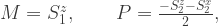
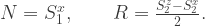
By calculating the mean values, we find $\langle\psi|MP|\psi\rangle=\frac{1}{\sqrt{2}}$ , $\langle\psi|NP|\psi\rangle=\frac{1}{\sqrt{2}},$ $\langle\psi|NQ|\psi\rangle=\frac{1}{\sqrt{2}},$ $\langle\psi|MQ|\psi\rangle=-\frac{1}{\sqrt{2}}.$ Then,

$\langle\psi|MP|\psi\rangle+\langle\psi|NP|\psi\rangle+\langle\psi|NQ|\psi\rangle-\langle\psi|MQ|\psi\rangle=2\sqrt{2}!$ (7)

Eq. (7) shows that the mean values taken over the state $|\psi\rangle$ do not obey Eq. (4)! However, this still proves nothing. Thus far we have only made algebraic calculations, in order to know which result is actually correct, we have to perform measurement in the real world. Many independent experiments have been conducted since the 1970’s in order to prove (or disprove) Bell’s and CHSH’s inequalities, and the amazing thing is that classical inequalities such as Eq. (4) are violated by physical systems! Experimental evidence strongly support Quantum Mechanic’s description of nature, and this means that if Quantum Mechanics is correct, then one (or more) of the following assumptions (made to obtain Eq. (4)) are incorrect:

Realism assumption: this is EPR’s assumption stating that the physical observables M, N, P and Q have definite values existing independently of observation.
Locality assumption: the assumption that Bob’s measurement does not influence Alice’s measurement (and vice-versa).

Together, these two are known as local realism and they played a fundamental role in EPR’s argument. Nowadays, many physicists believe that either one or both of them have to be discarded. By dropping the first assumption we have to acknowledge that physical properties do not have an existence independent of observation, and by discarding the second one we are considering that entanglement’s spooky action at a distance is an actual part of nature. The conflict between quantum entanglement and local realism is usually named non-locality of Quantum Mechanics.

Bell’s inequalities thus prove that Quantum Mechanics description of reality is complete and that the theory is non-local.

Hidden Variables Theories

Without getting into too much detail, I want to mention Hidden Variable Theories as they played an important role during the years in between EPR’s and Bell’s paper. As we already mentioned, Einstein believed that Quantum Mechanics’s wave function description of reality was incomplete, and it seemed that this problem could be solved by considering a set of theories called Hidden Variable Theories. In these theories, measurements are actually deterministic but appear probabilistic due to the existence of unknown degrees of freedom. Therefore, if Quantum Mechanics could not determine said hidden variables it would be a incomplete theory.

Many Hidden Variable theories were developed in the early and mid 1900’s, and it was Bell who proved that no physical theory of local hidden variables can ever reproduce all of the predictions of Quantum Mechanics.

For further reading about Bell’s Inequalities, I recommend reading his paper, I also found this article very useful. The CHSH inequality I presented was taken from Nielsen and Chuang’s book “Quantum Computation and Quantum Information”.

Entanglement (II): Non-locality, Hidden Variables and Bell’s Inequalities. by Marco Vinicio Sebastian Cerezo de la Roca is licensed under a Creative Commons Attribution-NonCommercial-ShareAlike 4.0 International License.

5 Responses to Entanglement (II): Non-locality, Hidden Variables and Bell’s Inequalities.

tonyr says:

22 June, 2015 at 4:02 pm

Reblogged this on tonyr and commented:

Great summary of a concept that plagued my understanding of quantum systems for years! Hidden variables always felt more satisfying, at least superficially, but you can’t argue with Bell on this one.

Alan Forrester says:

22 June, 2015 at 4:43 pm

Quantum mechanics is entirely local. The Bell inequalities imply that if quantum systems are described by stochastic variables, then the resulting description must be non-local. But quantum systems are described by Heisenberg picture observables, not stochastic variables. The equations of motion of real quantum systems are local, and as a result the patterns of dependence among Heisenberg picture observables are local,as explained in these papers:

http://arxiv.org/abs/quant-ph/9906007

http://arxiv.org/abs/1109.6223.

- marcocerezo says:
  
  22 June, 2015 at 4:53 pm
  
  Thank you very much for commenting and sharing. I’ll be sure to read the articles you linked!
  
Philomath says:

23 June, 2015 at 10:36 am

Great blog. Quantum entanglement is about he most unintuitive measurement/observation I can think of in Physics. Every atom in my body tells me that there must be underlying variables, yet experiments seem to have proven without a doubt that there isn’t. I will have to just accept the atoms in my body have not been observed yet lol (Joke)

On the serious side of this fascinating phenomena, I can only assume we have a lot more to learn. Describing something is not explaining it, and we are far from explaining quantum entangled particles, quantum superposition, and basically that particles of which everything we know is made of, do not actually exists until observed.

Previously my thoughts were the measurement instrumentation interfere with the quantum wave, physically, and disrupts it collapsing the wave function, thus bringing about a definite position. But after reading some of the ”Delayed choice quantum eraser” experiments, I am now even more confused.

It seems to me, and correct me if I’m wrong, but the experiment, the particle to be precise, knows in advance whether measurement will be made or not, and acts as a wave or particle depending on future action, going back in time or having advance knowledge.

My questions are: who is considered an observer, does time actually flow at this scale, and could this mean Everett’s “many worlds interpretation”, could actually be the most logical? and am real when I’m alone? do I have to see people to actually exist.

I have tried explain my ignorance about this subject in one of my blogs. link below.

http://swarmverdict.com/2015/01/09/quantum-weirdness/

George Rajna says:

23 June, 2015 at 5:03 pm

https://www.academia.edu/12559319/How_Time_Emerges_from_Quantum_Entanglement